Exponentially Weighted Moving Averages and MACD
What is EWMA?
A moving average takes a noisy time series and replaces each value with the average value of a neighborhood about the given value. This neighborhood may consist of purely historical data, or it may be centered about the given value. Furthermore, the values in the neighborhood may be weighted using different sets of weights. Here is an example of an equally weighted three point moving average, using historical data,
Here, $s_{t}$ represents the smoothed signal, and $x_{t}$ represents the noisy time series. In contrast to simple moving averages, an exponentially weighted moving average (EWMA) adjusts a value according to an exponentially weighted sum of all previous values. This is the basic idea,
This is nice because you don’t have to worry about having a three point window versus a five point window, or worry about the appropriateness of your weighting scheme. With the EWMA, previous perturbations “remembered”, and “slowly forgotten”, by the $s_{t-1}$ term in the last equation, whereas with a window or neighborhood with discrete boundaries, a perturbation is forgotten as soon as it passes out of the window.
How do I do this in code?
This code assumes that you have a Pandas DataFrame with a price column, and
a datetime column. The following code creates two columns, ewm_12 and
ewm_26 using the Pandas’ ewm method, and the span argument. This will
create exponential moving averages over 12 and 26 day windows, respectively.
From there, we can calculate the Moving Average Convergence/Divergence curve by
taking the difference of the ewm_12 and ewm_26 curves. From there, the MACD
Signal is the 9 day window exponential moving average of the MACD curve.
import matplotlib.pyplot as plt
import pandas
import seaborn

# build mkt dataframe with 'price' and 'datetime' columns

mkt['ewm_12'] = mkt['price'].ewm(span=12).mean()
mkt['ewm_26'] = mkt['price'].ewm(span=26).mean()
mkt['macd'] = mkt['ewm_12'] - mkt['ewm_26']
mkt['macd_signal'] = mkt['macd'].ewm(span=9).mean()
mkt['macd_minus_signal'] = mkt['macd'] - mkt['macd_signal']
From here, we can plot the price curve, and the exponential moving average
curves.
m = mkt[['price', 'ewm_12', 'ewm_26']]
axes = seaborn.lineplot(data=m, color='k')
axes.grid(True)
plt.xticks(rotation=45)
plt.show()
plt.savefig('exponential-moving-average.png', dpi=200)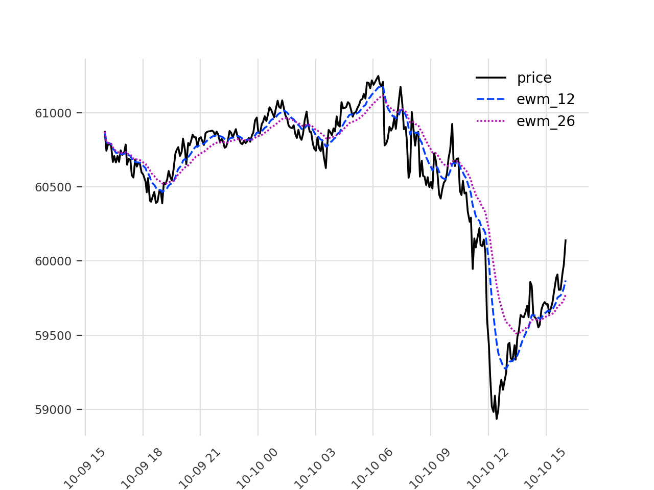
Here, we can plot the MACD curve, and the difference between the MACD curve and the MACD Signal curve. One interpretation of this difference is that negative values suggest a bear market, while positive values suggest a bull market.
m = mkt[['macd', 'macd_signal', 'macd_minus_signal']]
axes = seaborn.lineplot(data=m, color='k')
axes.grid(True)
plt.axhline(y=0, color='k', linestyle='-')
plt.xticks(rotation=45)
plt.show()
plt.savefig('macd-signal.png', dpi=200)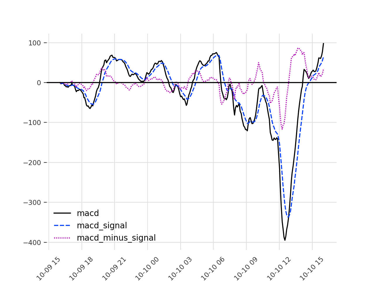
Conclusion
By incorporating EWMA and MACD into your technical analysis, you gain valuable insights into price movements. While not foolproof, these indicators can help you identify trends, potential reversals, and even trading signals. Remember, they are just one piece of the puzzle, and a well-rounded trading strategy considers other factors too.